OME-NGFF Images

OME-NGFF is a convention for storing bioimaging data in Zarr. A microscopy image is often far too large to open at full resolution, so an OME-NGFF store holds the same image several times over at decreasing resolutions — an image pyramid — and records the arrangement in group attributes. Reading one means consulting those attributes to pick a resolution, then reading the array it points to.

The convention is independent of where the store lives. This vignette reads a local store and a remote one with the same code; only the store object differs. See vignette("remote-stores") for connection details.

The multiscales attribute

The root group carries a multiscales attribute describing the pyramid. Each entry in its datasets list names a path within the store, ordered from highest resolution to lowest:

root <- pizzarr_sample("dog.ome.zarr")

g <- zarr_open_group(DirectoryStore$new(root))

attrs <- g$get_attrs()$to_list()
names(attrs)
#> [1] "multiscales" "omero"

vapply(attrs$multiscales[[1]]$datasets, function(d) d$path, character(1))
#> [1] "0" "1" "2" "3" "4"

Those paths are the arrays. Taking the first gives full resolution:

first_resolution <- attrs$multiscales[[1]]$datasets[[1]]$path

zarr_arr <- g$get_item(first_resolution)
zarr_arr$get_shape()
#> [1]   3 500 750

Three channels of 500 by 750 pixels — RGB. Reading it all and plotting takes the array into the channel-last order rasterImage() expects:

arr <- zarr_arr$get_item("...")$data

dm <- dim(arr)
plot.new()
plot.window(c(0, dm[3]), c(0, dm[2]), asp = 1)
rasterImage(aperm(arr, c(2, 3, 1)) / 255, 0, 0, dm[3], dm[2])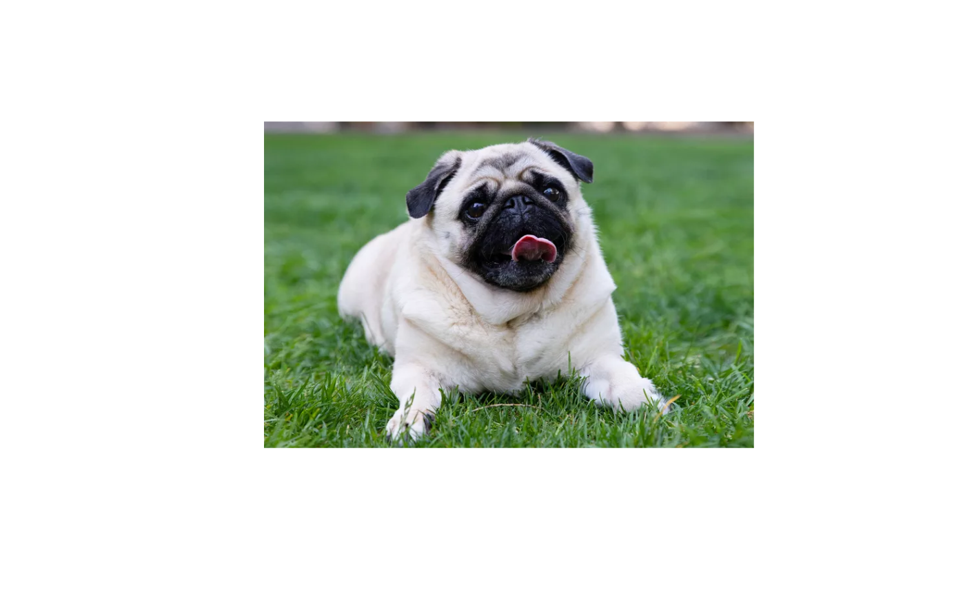

The same code against a remote store

A published OME-NGFF image behaves identically — swap DirectoryStore for HttpStore and nothing else changes. This one comes from the EMBL-EBI Image Data Resource, which serves its Zarr over an S3-compatible endpoint:

g <- zarr_open_group(HttpStore$new(idr_url))

attrs <- g$get_attrs()$to_list()
first_resolution <- attrs$multiscales[[1]]$datasets[[1]]$path

zarr_arr <- g$get_item(first_resolution)
zarr_arr$get_shape()
#> [1]   2 236 275 271

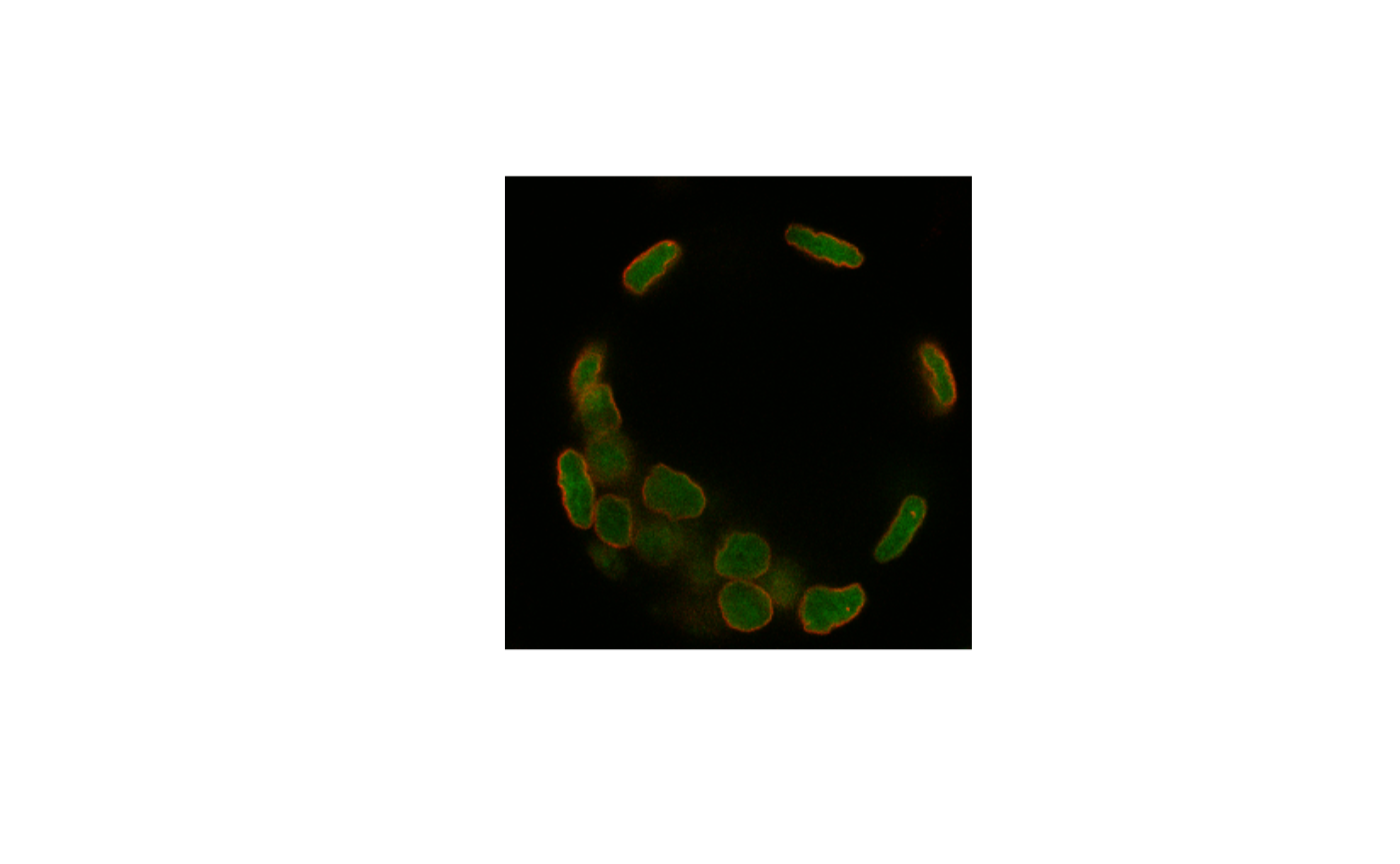
This image has four dimensions — two channels, 236 Z-planes, then 275 by 271 pixels. Reading all of it would pull far more than the illustration needs, so take a single Z-plane. Only the chunks overlapping the selection are fetched:

z_index <- 118

nested_arr <- zarr_arr$get_item(list(
  slice(1, 2), slice(z_index, z_index), slice(NA, NA), slice(NA, NA)
))

nested_arr$shape
#> [1]   2   1 275 271

The two channels are not red and green as such — they are separate stains. Mapping them onto two colour channels gives a quick look:

arr <- nested_arr$data

rg_arr <- aperm(arr, c(2, 4, 3, 1))[1, , , ]
rgb_arr <- array(0, dim = c(271, 275, 3))
rgb_arr[, , 1] <- rg_arr[, , 1]
rgb_arr[, , 2] <- rg_arr[, , 2]

plot.new()
plot.window(c(0, 271), c(0, 275), asp = 1)
rasterImage(rgb_arr / max(rgb_arr), 0, 0, 271, 275)